The impact of multiple structural changes on mortality predictions

Mortality models are calibrated using historical mortality data and mortality projections are obtained by projecting mortality trends into the future. In most of the recent literature the observed mortality trends are linear. However, if we calibrate the mortality rate on a longer period, the linearity assumption may no longer hold. This article illustrates a method to identify changes in the historical mortality trends. Using this method, projections of mortality rates can be based on the most recent mortality trend. We show that this leads to robust projections that connect better with recent mortality observations. [1] [2]

Introduction

Life insurance companies and pension funds need to monitor and predict mortality improvements for proper pricing and reserving. The last few decades mortality improved substantially, but these improvements were not stable over time. If we calibrate our model on a longer time span, the more likely it is that there has been one or even more structural changes in mortality (trends). In this article we describe a method that allows us to identify structural changes in mortality trends. We illustrate this method by calibrating the Lee-Carter model to Dutch male mortality data and by checking for structural changes in the estimated mortality trend.

Definitions and mortality models

Before we can estimate a mortality model and use that to make mortality projections, we need to define some variables. Let D_t,x be the number of deaths aged x in calendar year t and the average population aged x during calendar year t be E_t,x.(the exposure), with x ∈ {x₁, … , x_N} and t ∈ {1, …, T}. Further, define the death rate m_t,x­ = D_t,x/E_t,x. 

Lee and Carter [1992] introduced the first stochastic mortality model. The death rates are assumed to be a function of two age effects (βⁱ_x) and one period effect (κ²_t):

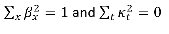
Lee and Carter estimate the parameters β¹_x, β²_x and κ²_t using Singular Value Decomposition (SVD). Two parameter restrictions are imposed to uniquely identify the model, namely

Given these restrictions, β¹_x equals the average and log)mortality rate for age x. The product of β²_x and κ²_t denotes the age-dependent change in mortality. Lee and Carter use a random walk with drift process (RWD) to project the time series . Projections of κ²_t are used to construct mortality rate projections. The process is specified by:

Given a time series , we can estimate the drift parameter δ as follows

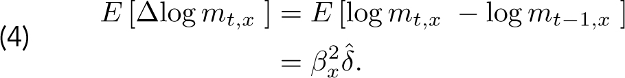
The expected change in mortality for age x from year t-1 to year t equals

In the Lee-Carter model, the variance of the mortality rate depends on the parameter . However, there is no dependency between the variance of the mortality rate on one hand, and the level of the mortality rate or exposure of a particular age on the other. To loosen this restriction, Brouhns et al. [2002] assume the observed mortality counts D_t,x are Poisson distributed: . In this specification, the variance in the death counts is proportional to the exposure and the mortality rate. The parameters can be obtained using numerical optimization methods such as Newton-Raphson.

In the Lee-Carter model mortality rates at all ages are perfectly correlated as there is only one time-dependent variable that influences the mortality rates. There are several extensions of the Lee-Carter model that produce a non-trivial correlation structure in mortality rates. Examples are the introduction of multiple period effects (Cairns et al. [2006], Plat [2009]), the introduction of a cohort effect (γ_t-x) (Renshaw and Haberman [2006]), and the introduction of period effects for specific age groups. (Plat [2009], O’Hare and Li [2011]). This article covers only the projection of period effects; the illustrations provided are obtained using the Lee-Carter model with Poisson distributed death counts.

Projection of period effects

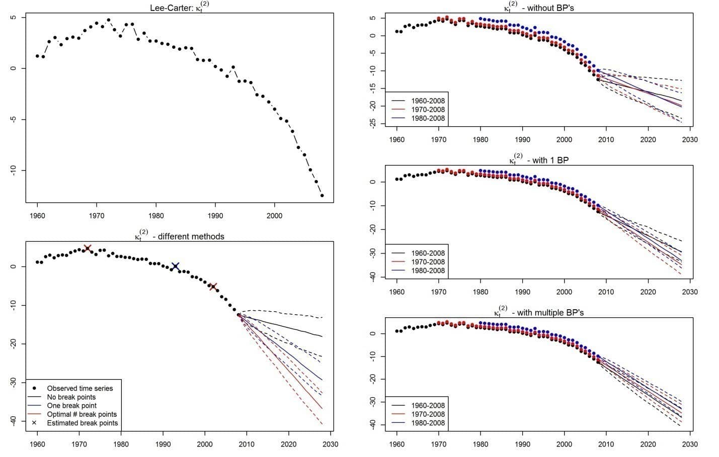
The random walk with drift model defined in (2) is the model that is most commonly used to project period effects in mortality models. From (3) it is clear that δ^{^} and the resulting projections of κ_t for t > T can strongly depend on the calibration period. Therefore, projected mortality changes can also strongly depend on the calibration period. Figure 1 shows the estimated time series κ_t for different calibration methods as well as projections based on a range of periods using the RWD model. This figure indicates that it is not likely that the drift parameter is constant over time.

It is desirable that the projections of the time series are less dependent on the calibration period and that the projections better connect with recent observations. To achieve this goal, we need to introduce a random walk with time-dependent drift process.

Structural changes in period effects

In the standard RWD model the drift parameter δ is constant over time. In our model this parameter is constant during a certain period of time, but may differ from period to period. This can be shown as follows:

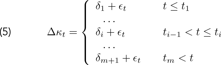
The δ_i are time-dependent drift parameters and the t_i are points in time at which a structural change occurs (hereafter: break points). We limit the possible break points with the restriction t_i – t_i-1 ≥ 5, which means that a trend continues for at least five years. In the random walk with time-dependent drift process we estimate three types of parameters: the number of structural changes (m), the break points (t_i), and the drift parameters in the periods between two consecutive break points.

We cannot estimate these parameters simultaneously. Therefore, we estimate one parameter at a time while keeping all others fixed,

Given the number of structural changes (m) and the break points (t_i), we can estimate the drift parameters δ_i by minimizing the sum of squared residuals (SSR):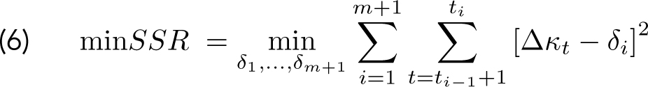

Since we do not know the break points in advance we have to estimate these. Given m, we can calculate the SSR for all combinations . The combination of break points that lead to the smallest SSR is considered optimal.

To determine the optimal number of structural changes, we use the Bayesian Information Criterion (BIC). The BIC provides a way to determine the quality of a model in terms of fit and the number of parameters needed to obtain the fit:

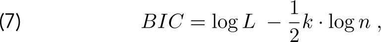
in which log L the log-likelihood of the model, k is the number of parameters in the model and n is the number of observations. The higher the BIC, the better the quality of the fit given the number of parameters (the second term in the right-hand side of (7) is a penalty for the number of parameters used).

In this article we estimate the time-dependent RWD for m ∈ {0, …, 5} and compute the corresponding BIC(m) . The optimal number of structural changes (m*), is then determined as

Given the framework above, we can estimate the RWD model with a time-dependent drift parameter. Using the latest drift δ^{^}_m+1 and the last observation κ_t we can simulate the period effect and project mortality rates. In the following paragraph we illustrate this using the Lee-Carter model.

Structural changes in the Lee-Carter model

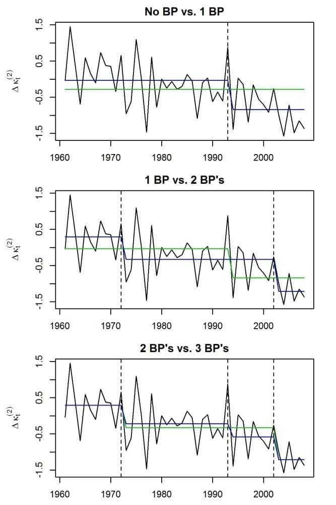
In this example we look at Dutch males aged 60-89. For the calibration period 1960-2008, the estimated period effect is shown in the top left graph in Figure 1. For this dataset it seems unlikely that the drift parameter is constant over the entire period; there seem to be structural changes around the years 1970 and 2000. Figure 2 shows the first differences of the time series (Δκ_{t =} κ_t – κ_t-1), and the average appears to be non-constant which indicates a time-dependent drift. The bottom left graph in Figure 1 shows the projected time series. The black lines show the projection when structural changes are not taken into account. This projection does not connect well with the historical observations.

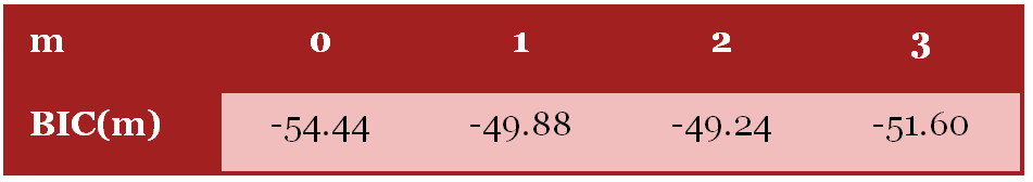
Figure 2 shows the optimal δ_i’s, given (m) or (m+1) structural changes for m ∈ {0,1,2}. The green and blue lines represent the estimated δ using (m) respectively (m+1) structural changes. In general we observe that when we allow more structural changes, the fit of the model increases. The improvement in fit from two to three structural changes is limited and based on the BIC the model with two structural changes is optimal as shown in Table 1.

Summary

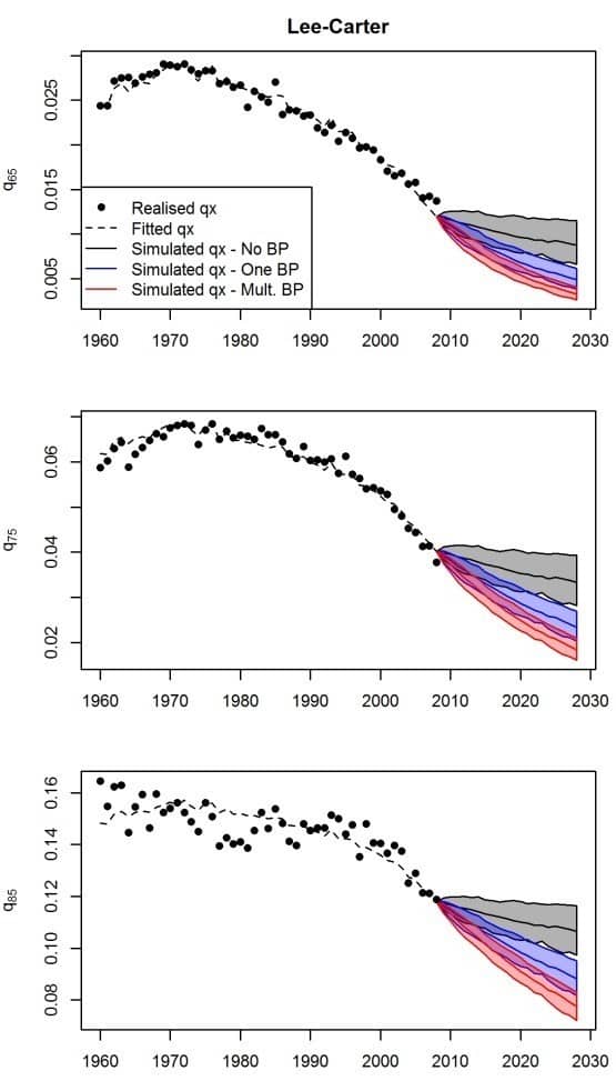
The bottom left graph of Figure 1 shows projections of the period effect calibrated in the period 1960-2008 for different numbers of structural changes. The projections are considerably better when structural changes in the past are taken into account. Further, the graphs on the right in Figure 1 show that projections are less dependent on the calibration period when structural changes are allowed. Moreover, the results show that it is necessary to allow for not one, but multiple structural changes. Figure 3 shows the projections of mortality rates while allowing for different numbers of structural changes. The black surfaces show projections without structural changes and these do not connect well with the latest observations. The blue and red surfaces connect better with recent observations. Based on BIC, two structural changes (in red) are optimal, and therefore we have to allow for multiple structural changes when projecting mortality using the Lee-Carter model on this dataset [3]. If we would not allow for structural changes, we would underestimate mortality improvements.

When a model is estimated on a historical dataset in order to make projections, it is of great importance to investigate whether the parameters are constant over time. This article describes a way in which structural changes can be identified within a dataset. We illustrate this method using the Lee-Carter model, and we show that mortality projections based on the latest mortality trend connect better with recent observations than when structural changes are not allowed. Not allowing for structural changes would in this case lead to an underestimation of mortality improvements.

Frank van Berkum is a senior consultant at PwC and a PhD student at the University of Amsterdam. In case you have any questions regarding this article, or regarding working at PwC, you can contact him via frank.van.berkum@nl.pwc.com or +31 6 5395 8614. 

[1] This article is based on the paper “The impact of multiple structural changes on mortality predictions” (http://dx.doi.org/10.1080/03461238.2014.987807, forthcoming in Scandinavian Actuarial Journal) by Frank van Berkum, Katrien Antonio and Michel Vellekoop, all affiliated with the University of Amsterdam. Antonio is also affiliated with the KU Leuven and Van Berkum and Vellekoop are also affiliated with Netspar.
[2] References are available upon request by the author (f.vanberkum@uva.nl).
[3] See our online article for back testing results; these confirm the necessity of allowing for multiple structural changes.