What Is the Pooling Problem?

July 12, 2016July 12, 2016 Nekst-Online 397 Views

The pooling problem is well-studied in the chemical process and petroleum industries. It is a generalization of a minimum cost network flow problem where products possess different specifications. The goal of solving a pooling problem is to find the lowest cost flow-rates in the network that satisfy the demands. In this essay, a mathematical model of a pooling problem, called the P-formulation [6], is studied and the different approaches to solve these types of problems are mentioned.

Introduction

The pooling problem, which is a subproblem of wastewater networks, crude oil refinery planning, etc, is important because of the huge amount of money that can be saved by solving it to optimality. In a pooling problem, flow streams from different sources are mixed in intermediate tanks (pools) and blended again in the terminal points. At the pools and terminals, the quality of a mixture is given as the volume (weight) average of the qualities of the flow streams that go into them.

In the pooling problem, there are three types of tanks: inputs or sources, which are the tanks to store the raw materials, pools, which are the places to blend incoming flow streams and make new compositions, and outputs or terminals, which are the tanks to store the final products. According to the links among different tanks, pooling problems can be classified into three classes:

Standard pooling problem: In this class there is no flow stream among the pools. It means that the flow streams are in the form of input-output, input-pool and pool-output; see Figure 1.
Generalized pooling problem: In this class, the complexity of the pooling problem is increased by allowing flow streams between the pools.
Extended pooling problem: In this class, the problem is to maximize the profit (minimize the cost) on a standard pooling problem network while complying with constraints on nonlinearly blending fuel qualities such as those in the Environmental Protection Agency (EPA) \textit{Title 40 Code of Federal Regulations Part 80.45}.

Figure 1: An example of a standard pooling problem with I inputs, L pools and J outputs.

There are many equivalent mathematical formulations for a pooling problem, such as P-, Q-, PQ- and HYB- formulations, and all of them are formulated as a nonconvex (bilinear) problem, and consequently the problem can possibly have many local optima. These formulations vary in the way of representing specifications in the pools. For instance, in the Q-formulation the fraction of incoming flow to a pool that is contributed by an input is considered.

P-Formulation

For each arc $(i,j)\in \mathcal{A}$ , let $c_{ij}$ be the cost of sending a unit flow on this arc. For each node, there is possibly a capacity restriction, which is a limit for sum of the incoming (outgoing) flows to a node. The capacity restriction is denoted by $C_i$ for each $i\in N$ . Also, there are some specifications for the inputs, e.g. the sulfur concentrations in them, which are indexed by $k$ in a set of specifications $\mathcal{K}$ with $K$ members. By letting $y_{ij}$ be the flow from node $i$ to node $j$ , $u_{ij}$ the restriction on $y_{ij}$ that can be carried from $i$ to $j$ , and $p_{lk}$ the concentration value of $k$ th specification in the pool $l$ , the P-formulation of a pooling problem can be written as the following optimization problem:

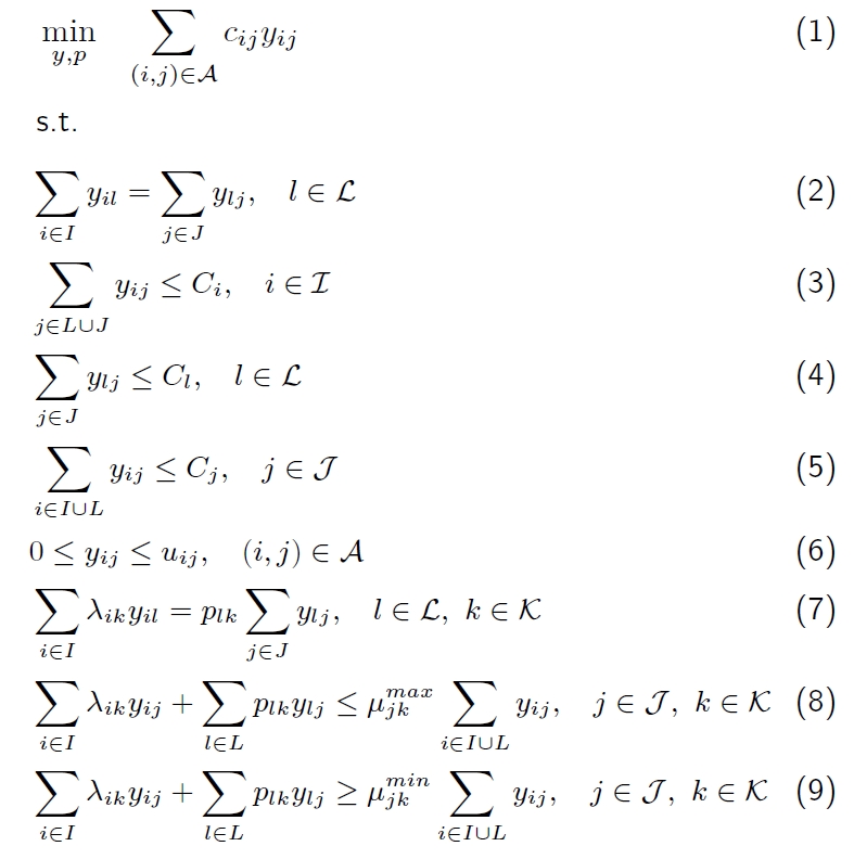
where $\mu^{max}_{jk}$ and $\mu^{min}_{jk}$ are the upper and lower bound of the $k$ th specification in output $j\in \mathcal{J}$ , and $\lambda_{ik}$ is the concentration of $k$ th specification in the input $i$ . Here is a short interpretation of the constraints:

(2): The pools are just for mixing the incoming flow streams, and nothing is stored in them. So, the total flow-rates going into any pool goes out from the pool.

(3), (4), (5): The inputs, outputs and pools are specific tanks. Hence, they have some capacity restriction in order to store a raw material or product, or to mix some flow streams.

(6): The links in the networks represent devices that carry flows from one unit to the others (for instances, pipes). So, this constraint is due to the capacity limits on these devices.

(7): The concentration of any specification in each pool is the average of the concentrations of the specification of the incoming flow streams. In other words, for the $k$th specification in the pool $l$ ,

$\begin{equation*} p_{lk}=\frac{\sum_{i\in \mathcal{I}}\lambda_{ik}y_{il}}{\sum_{i\in \mathcal{I}}y_{il}}. \end{equation*}$

(8), (9): As was mentioned, in addition to the pools, the flow streams are mixed in the outputs as well. Therefore, for each output $j$ and specification $k$ , the concentration is

$\begin{equation*} p_{jk}=\frac{\sum_{i\in \mathcal{I}}\lambda_{ik}y_{ij}+\sum_{l\in \mathcal{L}}p_{lk}y_{lj}}{\sum_{i\in \mathcal{I}}y_{ij}+\sum_{l\in \mathcal{L}}y_{lj}}. \end{equation*}$

But for the outputs, there are usually some restrictions on the concentration of each specification. These restrictions appear as lower and upper bounds. So,

$\begin{equation*} \mu^{min}_{jk}\leq \frac{\sum_{i\in \mathcal{I}}\lambda_{ik}y_{ij}+\sum_{l\in \mathcal{L}}p_{lk}y_{lj}}{\sum_{i\in \mathcal{I}}y_{ij}+\sum_{l\in \mathcal{L}}y_{lj}}\leq \mu^{max}_{jk}. \end{equation*}$

More information about different formulations can be found in [5].

Solution methods and softwares

Despite the strong $\mathcal{NP}$ -hardness, which is proved in [2], much progress in solving small to moderate size instances to global optimality has been made from 1978 onward, when Harvely described the P-formulation and solved small standard pooling problems by a graphical view of them.

Regarding the solution of a pooling problem, there are many methods in the literature. In all methods, a lower and upper bound are proposed and a way of reducing the gap between them is studied. One way of getting a lower bound for a pooling problem is using convex relaxation, as done by Foulds et al. [4]. Moreover, Adhya et al. [1] introduce a Lagrangian approach to get a tighter lower bound for pooling problems. Recent work done by R. Misener et al. [8] uses a novel piecewise linear relaxation for the bilinear terms with a logarithmic number of binary terms; this is implemented to the software APOGEE in order to solve a pooling problem. The idea of relaxing bilinear terms is described here.

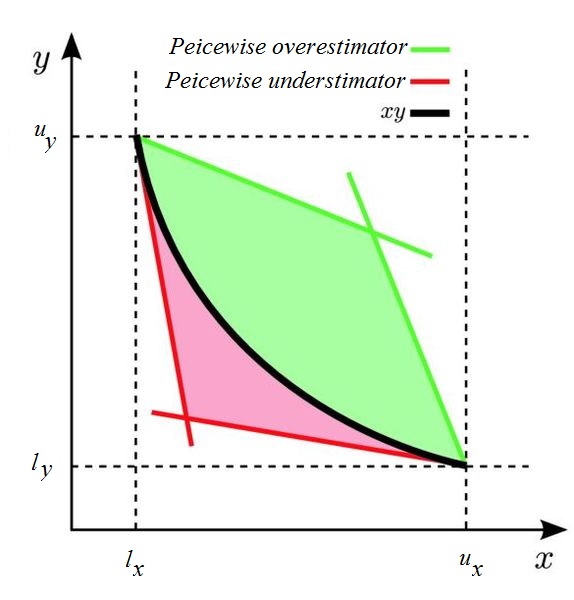
McCormick envelope

Assume that $x$ and $y$ are variables with given lower and upper bounds

$\begin{equation*} \ell_x \le x \le u_x, \;\;\; \ell_y \le y \le u_y. \end{equation*}$

Then, the following four inequalities are implied (Figure 2):

(1) $\begin{eqnarray*} xy &\ge & \ell_x y + \ell_y x - \ell_x \ell_y, \nonumber \\ xy &\ge & u_x y + u_y x - u_x u_y,\nonumber \\ xy &\le & \ell_x y + u_y x - \ell_x u_y,\nonumber \\ xy &\le & u_x y + \ell_y x - u_x \ell_y.\nonumber \end{eqnarray*}$

By substituting $xy$ with a new variable $w$ , we replace a 3-dimensional surface

$\begin{equation*} \left\{(x,y,xy):\; \ell_x \le x \le u_x, \;\;\; \ell_y \le y \le u_y\right\} \end{equation*}$

by the convex set

$\begin{align*} C=\bigg\{(x,y,w):\; \ell_x \le x \le u_x, \;\;\; \bigg.& \ell_y \le y \le u_y,\;\;\; \\ & \left. \begin{matrix} w \ge \ell_x y + \ell_y x - \ell_x \ell_y \\ w \ge u_x y + u_y x - u_x u_y\\ w\le \ell_x y + u_y x - \ell_x u_y\\ w \le u_x y + \ell_y x - u_x \ell_y \end{matrix} \right\} \end{align*}$

It is clear that $C$ , called the McCormick envelope [5], is a polytope and the surface lies in it.

In the pooling problem (1), it is clear by the structure that:

$\begin{matrix} \min_{i\in \mathcal{I}}\lambda _{ik}\leq p_{lk} \leq \max_{i \in \mathcal{I}}\lambda _{ik},& \hspace{.5cm}\forall l\in \mathcal{L},\; k\in \mathcal{K},&\\ 0\leq y_{lj} \leq C_j, &\hspace{.5cm}\forall j\in \mathcal{J},\; l\in \mathcal{L}.& \end{matrix}$
So, one can replace each $p_{lk}y_{lj}$ that appears in (1) by its McCormick envelope to get a piecewise linear relaxation.

Figure 2: McCormick envelope: the union of red and green sets

To make the McCormick envelope tighter, one can split the intervals $\ell_x \le x \le u_x$ and $\ell_y \le y \le u_y$ into many intervals and construct the McCormick envelope for each pair of intervals on $x$ and $y$ .

Furthermore, there is another software package, called GloMIQO [7], in which a pooling problem can be solved by generating tight convex relaxations, partitioning the search space, bounding the variables, and finding good feasible solutions.

References

[1] N. Adhya, M. Tawarmalani, and N. V. Sahinidis. A Lagrangian approach to the pooling problem. Industrial & Engineering Chemistry Research, 38(5):1956–1972, 1999.
[2] M. Alfaki. Models and solution methods for the pooling problem. Ph.D. thesis, University of Bergen, 2012.
[3] S. S. Dey and A. Gupte. Analysis of MILP techniques for the pooling problem. Operations Research, 63(2):412–427, 2015.
[4] L. R. Foulds, D. Haugland, and K. Jörnsten. A bilinear approach to the pooling problem. Optimization, 24(1-2):165–180, 1992.
[5] A. Gupte, Sh. Ahmed, S. S. Dey, and M. S. Cheon. Pooling problems: relaxations and discretizations. Optimization Online, 2013.
[6] C. A. Haverly. Studies of the behavior of recursion for the pooling problem. ACM SIGMAP Bulletin, (25):19–28, 1978.
[7] R. Misener and Ch. A. Floudas. Glo{MIQO}: Global mixed-integer quadratic optimizer. J. of Global Optimization, 57(1):3–50, 2013.
[8] R. Misener, J. P. Thompson, and Ch. A. Floudas. APOGEE: Global optimization of standard, generalized, and extended pooling problems via linear and logarithmic partitioning schemes. Computers & Chemical Engineering, 35(5):876–892, 2011.

Text by: Amadreza Marandi

Introduction

P-Formulation

Solution methods and softwares

McCormick envelope

References

You May Also Like

Over-The-Counter Trades in Longevity Risk

Life Cycle Behavior Under Prospect Theory Preferences

Humanitarian logistics optimization