Create and Enrich Road Networks for Optimization Using OpenStreetMap and GPS Traces

April 15, 2021April 29, 2021 Nekst-Online 276 Views Network, Optimization, Road Networks

One of the prerequisites of successfully applying Operations Research techniques is having the right data available. As an example, when applying a shortest path algorithm, we need to know the underlying graph network for the results to make sense. If not all edges are present in this graph, the shortest path may not be as optimal as we would think or hope. In this article, we focus on finding an accurate representation of a road network, which can be used for optimizing, for instance, routing decisions. Written by: Valentijn Stienen

Introduction
An accurate representation of a road network is essential when performing network analyses. We can often rely on maps such as OpenStreetMap (OSM) and Google Maps for these representations. However, this is not always the case. For instance, in remote areas, roads may not exist in OSM or are not accurately connected with each other. This might lead to significant flaws in optimal routing decisions that are based on these road networks.

To be able to complement such road networks, we can use GPS trajectories. Equipping vehicles with GPS trackers results in lots of data about the location of a vehicle along with its course and current speed. This information tells us, for instance, that a vehicle has been driving on road $X$ with velocity $Y$ at time $Z$ . If a vehicle drives a particular route, the tracker returns an ordered sequence (with respect to time) of such GPS points, which is called a GPS trajectory. We will discuss one way to create and complement road networks using such GPS trajectories. The final graph (result) should be suitable for optimization and navigation purposes.

Problem definition
We want to be able to optimize routing decisions in an area for which the road network is not completely known. We do, however, have GPS trajectories becoming available each day of vehicles that drive around in this area. Table 1 shows a sample of such data.

Table 1: Sample of GPS trajectory data on a particular day.

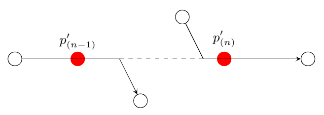
Now, the goal is to get an accurate representation of the road network. Let us first describe what this means mathematically. We want to end up with a graph object, say $G = (V,E)$ , where $V$ represents the set of nodes of $G$ , and $E$ the set of edges of $G$ . Additionally, we need to be able to extract information about the geometry of the road. This can be used to find actual distances (and later on, travel times), but it is also necessary for navigation purposes. When a driver navigates to his destination, we do not want to only point him in the direction of his next node (see Figure 1).

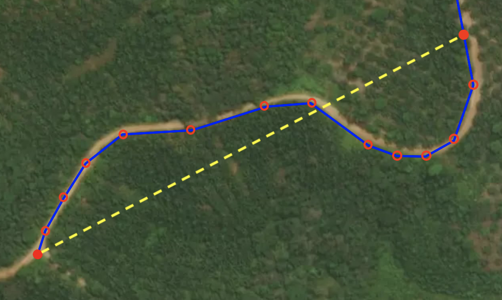
Figure 1: Information about how a road runs exactly (blue edge) should be in the graph. The yellow dashed line is notappropriate for navigation purposes.

One way to do this is to add a node for each point the road changes its course (the open red circles in Figure 1). However, this increases the number of nodes/edges of the graph significantly, which is not preferable due to computational reasons. Instead, we use the geometry of a road as an attribute of an edge. In particular, we use so-called linestrings to represent the geometries. A linestring is a path between two locations. It takes the form of an ordered series of at least two points. For instance, $\texttt{LineString((lat1, lon1),(lat2, lon2),}$ $\texttt{(lat3, lon3))}$ represents an edge that starts at the coordinate $\texttt{(lat1, lon1)}$ , then goes to $\texttt{(lat2, lon2)}$ and ends at $\texttt{(lat3, lon3)}$ . In this way, we only need one edge to represent the blue road in Figure 1. This means that for the nodes of $G$ , $V$ , we only include the intersection points of the roads. Points at which a driver can choose between at least two options. Additionally, we include end points of dead ends as nodes, as this might turn out to be a start or end location of a future origin-destination pair. For the edges of $G$ , $E$ , we include all possible roads between the nodes.

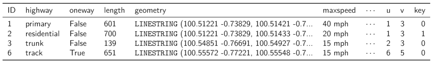
Table 2: Sample of the edges of a graph that represents a road network. Highway indicates the importance of the highway within the road network, and u(v) represents the ID of the start (end) node of this edge. Note that there may be multiple different roads (and therefore edges) between the same start and end point. These are distinguished using a key in the last column.

Initializing a first graph can be done using the information from OpenStreetMap. Using the work of Boeing [1], we are able to initialize a road network (graph) that has the features discussed above. He develops a method to easily extract the information from OSM into graph structures. In Table 2, we show a sample of how the edges of the graph are represented. In the rest of this article, we focus on how to extend this initial graph using the GPS trajectory information.

Approach
There are already several methods developed for generating road maps based on (solely) GPS trajectory data. For an overview and introduction of such map construction algorithms in general, we refer to the work of Ahmed et al. [2]. Instead of creating a new network, we discuss how to extend an existing network (based on OSM). Moreover, we need to take several specific restrictions into account. First, many roads that are in the trajectory dataset may not exist in the OSM database. Secondly, we need to take into account that the density of the GPS trajectories may be unevenly distributed. Some of the roads are more often used than other roads. Also, in general, there may not be much redundancy present on each road. We still want all roads that are driven only a few times to occur in our graph structure. Thirdly, we need to incorporate the sampling frequency (e.g., how much time passes between two consecutive GPS point locations). Finally, we prefer to use a method that easily adjusts the found network when additional GPS trajectories are obtained.

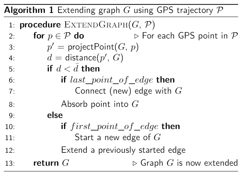
Incorporating these restrictions, one approach can be characterized as follows. We start with the initial graph and we subsequently consider GPS trajectories. For each trajectory, we extend the current graph. Let $\mathcal{P}$ be the ordered (with respect to time) set of GPS points, then the basic procedure is shown in Algorithm 1.

In the rest of this article, a GPS point will be denoted with $p_{(n)}$ , which represents the $n^{\text{th}}$ GPS point of $\mathcal{P}$ . Moreover, any projected point will be denoted with an apostrophe (e.g., $p_{(n)}'$ is the projected point corresponding to $p_{(n)}$ ). In the algorithm, we start with projecting the GPS point $p$ onto the current network (line 3), while incorporating the geometry of edges and the course of $p$ . Projecting means that we look for the point on the network that is closest to $p$ and is headed into a similar direction. Next, we compute the distance between $p$ and its projected point (line 4).

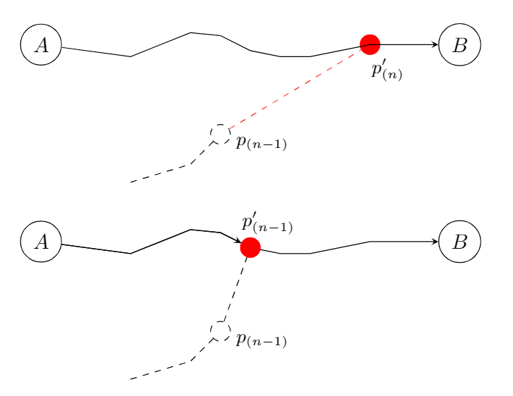
First, if this distance is small enough (impose a threshold, line 5), we absorb the point into the network (line 8). This means that we do not add any edges or nodes to the current network. However, there is one exception. For now, suppose that $p_{(n)}$ will connect a newly created edge to the network (last_point_of_edge, line 6). Note that this requires the previous point to not be absorbed into the network. In this case, we need to reconnect this new edge with the network (line 7). We illustrate this procedure in Figure 2.

Figuur 2: Connecting an edge with the network. Due to the fact that $p_{(n)}$ is absorbed in the network, we re-project $p_{(n-1)}$ onto the network to obtain the connection of the new edge with the current network.

The solid black line represents an edge from the current network. The dashed black line represents the edge that has been created up to this point. We are currently examining GPS point $p_{(n)}$ . Since this point is close to the network, we need to connect the new edge with the network. Instead of adding the red dashed line (illustrated in the top plot), we re-project the previous GPS point (which is part of the new edge to be created) onto the network, without incorporating the direction of this point. Then, we add this projected point, $p_{(n-1)}'$ , as node and we split the edge onto which this node exists $(A,B)$ into two edges: $(A, p_{(n-1)}')$ and $(p_{(n-1)}', B)$ . Finally, we add the new edge (dashed black lines) to the network (illustrated in the bottom plot).

Secondly, suppose the distance between the current GPS point and the projected point is not small enough (line 9). In this case, we must include this GPS point into a new edge. If this edge already exists, we extend it with this new point (line 12). If this is the first point in a sequence that cannot be absorbed (first_point_of_edge), we need to start a new edge (line 11). This can be done in a similar way as connecting a new edge with the network. We re-project the current point onto the network, without incorporating the direction, and we consider this point as the starting point of the new edge.

Based on this algorithm, we can extend a graph with multiple GPS trajectories sequentially. There are, however, still some things that can go wrong. Next, we discuss some potential drawbacks of this algorithm along with possible solutions for these drawbacks.

Missing roads
The first thing that can go wrong is that two consecutive points may be absorbed in the network, while there is no (direct) possibility to go from the first point to the second point in the current network. Such a situation is sketched in Figure 3.

Figuur 3: Example situation in which both $p_{(n-1)}$ and $p_{(n)}$ are absorbed into the network, but there is no direct connection from $p_{(n-1)}'$ to $p_{(n)}'$ .

A similar situation may occur when there is no (direct) connection from $p_{(n-1)}'$ to $p_{(n)}'$ in the example sketched in Figure 2. Therefore, we introduce another parameter that can be included into the projectPoint algorithm: close_to_edge. This parameter represents an edge that has to be close to the edge onto which we project a point. So when we project a point onto the network, we can use the fact that it must be projected onto an edge that is close to the close_to_edge. Note that close is defined per situation:

i) When $p_{(n-1)}$ was absorbed into edge $(A,B)$ , we prefer to project $p_{(n)}$ onto the same edge. If this is not possible, we would prefer projecting $p_{(n)}$ onto edges that leave node $B$ . If this is also not possible, we prefer to project onto edges leaving one of the endpoints of the edges leaving node $B$ , etc.

ii) Secondly, when $p_{(n)}$ starts a new edge, we define close as follows. Suppose $p_{(n-1)}$ was absorbed into edge $(A,B)$ of the current network. In this case, we prefer to project $p_{(n)}$ onto the same edge. If this is not possible, we would prefer projecting $p_{(n)}$ onto edges that leave node $B$ . If this is also not possible, we would prefer to project onto edges leaving one of the endpoints of the edges leaving node $B$ , etc.

iii) Finally, we define close when $p_{(n-1)}$ must connect a new edge with the current graph. Suppose $p_{(n)}$ (which is the last point of the edge) was absorbed into the network (into edge $(A,B)$ ). In this case, we want to project $p_{(n-1)}$ onto an edge that easily gets to $(A,B)$ , preferably $(A,B)$ itself. If this is not possible, we would prefer projecting $p_{(n-1)}$ onto edges that end in node $A$ . If this is also not possible, we would prefer to project onto edges ending in one of the start points of the edges ending in node $A$ , etc.

Connecting GPS trajectories
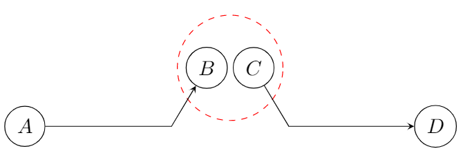
Besides the missing roads, we also need to be careful when having multiple GPS trajectories. If end or start points of trajectories are close to each other, we may need to combine these points into one node in order to ensure that a vehicle may pass this node. This situation is sketched in Figure 4.

Figuur 4: Example situation in which we merge node $B$ and $C$ into one node, in order to ensure that there is no disconnection between the two trajectories.

One trajectory has as final edge $(A,B)$ and one trajectory has as first edge $(C,D)$ . However, in this case, we are not able to move from $A$ to $D$ . To incorporate this information that multiple GPS traces could form a longer road, we build in a function that checks whether a point can be merged into another point. In the example in Figure 4, we combine $B$ and $C$ into one node, which ensures that we are able to move from $A$ to $D$ .

In conclusion, to be able to have a working algorithm, we need to know what could go wrong. Needless to say, this knowledge is often obtained when testing your algorithm for the first (or second, or …) time.

Case study
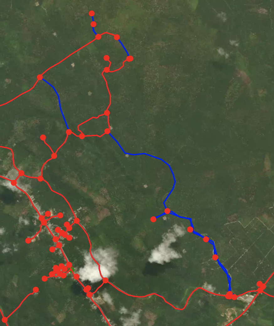
Finally, to check whether the proposed algorithm performs as expected, we try using it with some actual data. We create a small piece of a road network for a region in Indonesia for which we have GPS trajectories available of trucks transporting goods. We start with the OSM base map and run the algorithm for 11 GPS trajectories. The result is shown in Figure 5. We observe that some additional edges are added to the base map that will significantly affect the shortest paths between locations. Note that in the bottom right we see (if looking carefully) two parallel edges. Since all edges from the GPS trajectories are one-way only, these edges represent the two one-way edges running in opposite direction.

Next steps include predicting or learning the (actual) travel time of (new) edges based on the distance of an edge and the used speed of vehicles traversing this edge.

Figure 5: Result of extending the OSM base map (red edges) using the 11 GPS trajectories. Blue edges represent those edges added after running the algorithm.

References

[1] Boeing, G. (2017). OSMnx: New methods for acquiring, constructing, analyzing, and visualizing complex street networks. Computers, Environment and Urban Systems, 65, 126-139.

[2] Ahmed, M., Karagiorgou, S., Pfoser, D., and Wenk, C. (2015). Map Construction Algorithms. Springer.

You May Also Like

Humanitarian logistics optimization

The Optimal Wine Adventure

Estimation of Time Varying Partial Correlation Networks