

Optimizing the Blending of Malt at Holland Malt
Econometricians and beer, a combination almost as inseparable as babies and milk. Nearly every fellow econometrician has drunk a beer, and developed his own preference. While one likes the typical lager beers, another prefers a high fermentation specialty beer with a bitter after-taste. Whatever you may prefer, it likely has to do with the key ingredient of beer, called malt. Often, multiple malts are blended together to create a certain quality which is suitable for a particular brewery. The blending of these malts is a challenging task. In this article I will explain my model which optimizes the blends of malt, which is also the subject on which I wrote my master thesis at Holland Malt, a subsidiary of Bavaria.
Developing the model
The problem that I solved, is to create a proposal for the planner on how to blend the malts in stock for a certain target quality. A target quality is a list of properties on specifications and varieties imposed by a customer. A specification is a property of a malt, such as the “pH value”, while a variety determines the behavior of a malt during the brewing process. Malts are stored in silos to keep them from spoiling. When malts are blended they are transferred to delivery silos, from which they are dropped in a truck or transported to a ship. Now that the definitions are clear, the next step was to do research on other blending problems. Unfortunately, only the paper of Mutangi et al. [1] is found which deals with a blending problem in the malt industry. In other industries far more research is done, for example in the paper of Ashayeri et al. [2], where a model was made to solve the blending problem of a producer of chemical fertilizers. These papers provided insight on how to develop my model.
In order to create a suitable model, it is needed to know the exact restrictions of a blend. There are two types of restrictions which have to be met. Firstly there are the customer restrictions, which are requests on specifications and varieties of the delivered malt. Requests on specifications include bounds on the final mixture of malt, blending limits and aim values. Final mixture bounds mean that for example for the specification “Moisture”, representing the percentage of water in the malt, the value should be between 0 and 4.5 in the final blend. Blending limits are imposed to give a bound on the used malts in a blend. So for example malts with a value of 85 or lower for “Friability”, the crumbliness of malt, should not be used. Aim values determine a preferred value, such as a value of 1.55 for “viscosity”, called “stroperigheid” in Dutch. Also variety conditions are imposed by customers, such as whether the used malts may be spring or winter malts. More examples are the allowed number of different varieties and the minimum and maximum percentage of certain varieties used in the blend.
Secondly, there are company restrictions, which are divided in physical constraints and preferred conditions. An example of the first category is that silos from different silo blocks can not be used in the same blend, because it is physically impossible. But the most important physical restriction is about streams. A stream is a subset of silos which can replace one another. A maximum of four silos can be blended at the same time, and a blend has to stay homogeneous. Therefore, when one of the four used silos is emptied, a replacement silo has to take its place. This replacement silo has to be in the same stream, with maximally one other replacement silo. Since maximally four streams can be used, the total number of silos that can be used in a blend equals twelve. Check for yourself that this can only happen if eight silos are emptied. To model this a lot of artificial variables are needed, which is why it is not discussed furthermore in this article.
There are nine preferred conditions, also referred to as objectives. These include the amount of time malt is in a silo, the general quality of the malt, the reservation of the malt, the quantity of a silo, the number of empty silos, the violations on final mixture values, blending limits and aim values and the amount of used priority silos. These objectives often vary in importance per order, even for orders for the same target quality. One of the generally more important objectives is the reservation of malt, since some malts are reserved for certain target qualities, which are preferred not to be used for any other target quality.
In order to establish a solvable model which still approaches reality, multiple assumptions are needed. In total fourteen assumptions are made. One of those is that all specification values of a malt mixture are a linear function of the corresponding specification values of the individual malts. For some specifications, such as “Filtration speed”, this is not entirely true in practice. However, since large outliers in values are rare, this assumption is not that unrealistic. It also means a multi-objective mixed integer linear program can be solved.
Explanations of the model
The complete model uses around 2,500 variables and 50,000 constraints. These constraints are written in 67 different lines
Due to space restrictions only some are displayed and explained. The main variable in the model is xn, which indicates the percentage of malt taken from silo n. The first constraint makes sure the percentages of all silos sum up to 1.
The next two constraints define the relation between the binary variable yn and xn. When a positive percentage of silo n is taken (xn > 0), the value of yn is 1. When silo n is not used (xn = 0), then yn = 0. Moreover, these constraints make sure that when a silo is used (yn = 1), the value of xn must be at least a small positive number. The next constraint depends on Un. If Un = 0, it means that silo n may not be used in the blend (xn = 0). The following constraint is about the quantity of malt inside silos. The amount of kilogram taken from silo n, (AKO ∗ xn), should be smaller or equal than the amount of kilogram available in silo n.
The following constraints are all discussed in pairs. For some target qualities it is important to deliver for example a mix of 50% spring malt and 50% winter malt, meaning that the parameters MINZWd and MAXZWd should both be equal to 0.5. Note that ZWn is 1 if the malt in silo n is spring malt and 0 otherwise. So ![]() means that exactly 50% spring malt (and thus also 50% winter malt) is included in the solution.
means that exactly 50% spring malt (and thus also 50% winter malt) is included in the solution.
The next constraints contain violation variables, which are included in the objective of the problem, since violations on final mixture values, blending limits and aim values should be minimized. ![]() gives the value of speci- fication s in the final blend. Since it is preferable that this value is between the final mixture bounds
gives the value of speci- fication s in the final blend. Since it is preferable that this value is between the final mixture bounds
![]() , these constraints are included. Should it be impossible or non-optimal to remain within these bounds, the variable
, these constraints are included. Should it be impossible or non-optimal to remain within these bounds, the variable
![]()
becomes positive. The same kind of restrictions are needed for the aim values on specifications, for which deviations are generally less important than for final mixture values.
Next, the constraints on blending limits are provided. If silo n is used (yn = 1), the specification of the malt in silo n is preferred to be within blending limits
![]()
![]()
should this be optimal. Notice that if the value of either violation variable is positive for a certain specification, it is equal to the difference between the corresponding bound
![]() and the specification value of the used silo which deviates the most from this bound. The following constraints are included to take into account aim values on varieties. Notice that
and the specification value of the used silo which deviates the most from this bound. The following constraints are included to take into account aim values on varieties. Notice that
![]() gives the percentage used of variety r. Because RRrd∗ gives the preferred percentage of variety r for target quality d∗, these constraints make sure to approach the preferred percentages. The corresponding violation variables ensure that every variety percentage can occur, should this yield better results in the objective.
gives the percentage used of variety r. Because RRrd∗ gives the preferred percentage of variety r for target quality d∗, these constraints make sure to approach the preferred percentages. The corresponding violation variables ensure that every variety percentage can occur, should this yield better results in the objective.
The final constraints which are discussed in this smaller version of the complete model, make sure the physical restrictions on silo blocks are dealt with.
![]()
is 1 if all used silos are from silo block A, -1 if all used silos are from silo block B and C, and anywhere in between -1 and 1 otherwise. Since v is a binary variable, you can check for yourself that these constraints can only be both satisfied if
![]() is -1 or 1. This means that if silos from silo block A are used, no silos from B or C can be used, and vice versa. The remaining constraints are just non-negativity and binary constraints.
is -1 or 1. This means that if silos from silo block A are used, no silos from B or C can be used, and vice versa. The remaining constraints are just non-negativity and binary constraints.
Optimizing the model
The objective function of the complete model consists of multiple terms, including terms depending on the sum of violation variables. Each term is assigned its own objective weight. For equal objective weights, each term contributes an approximately equal share to the optimization process. However, by adjusting objective weights, one can give priority to for instance aim values for one target quality, while blending limits could be important for another.
The complete model also contains some objective constraints. These constraints can be used to get more control on the final solutions. For instance, an objective constraint is![]()
![]()
where M is a large number. This means that if β = 0, this constraint does nothing, while β = 1 means that the final mixture values must be satisfied.
In this way the objective terms depending on e1s and e2s do not contribute anymore, and the focus can be put on other objectives, given that the final mixture values are satisfied. Next to the provided model, multiple extensions were build. Examples are the usage of previous solutions and automation of input parameters. These extensions make sure that the quality and computation time of solutions increase greatly, which is the goal of using a model for this problem.
Results of the model
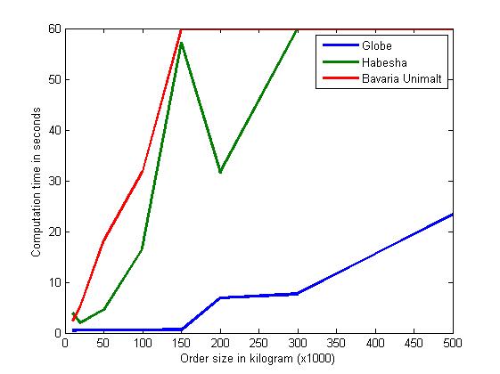
By blending manually, which was done until now, it could take around fifteen minutes of intensive work to generate a proper blend. Using this model requires less effort and reduces the computation time of most blends to less than ten minutes. Since multiple blends have to be made per day, using the model is indeed significantly time saving. Figure 1 shows that the correlation between the order size and computation time is quite high. This can be explained because of the stream constraints (not provided in this article). When an order increases in size, much more possible streams (silo combinations) can be used, which takes time to evaluate. Therefore, a small order of about 30.000 kilogram (30 ton) is often done in a matter of seconds, while large orders differ greatly in computation time per target quality.
The quality of a solution is difficult to measure, since a solution has many performance indicators. Of course the top priority is to satisfy the customer, but for instance emptying silos to be able to store new malt is often also very important. The model provides a way to generate a blend according to the users needs and should not be used by someone without the proper knowledge of the final solutions. Sometimes a solution seems good, while in fact the best malt in stock is used, which gives an enormous problem one week later. Therefore, at all times a close eye should be kept on the current inventory. A promising recommendation is to expand upon the provided model. The blending of malt is only one subproblem of the entire supply chain of Holland Malt. Calculating which barleys should be malted into malt, and which barleys to buy, is still not automated, and it would be very interesting to provide a model in these areas as well.
The planner at Holland Malt has already used the complete model with success. Multiple real-life optimizations are done and the solutions of most of these optimizations are actually used in practice. So now it is clear to me why econometricians and beer are inseparable. Not only because we enjoy drinking beers, but also because we are the ones who can develop and implement extensive mathematical optimization models in the beer industry.
References
[1] Mutangi,T., Nyanga, L., van der Merwe, A.F., Chikowore, T.C., Kanyemba,G. (2013). A Linear Programming Model For Blending. SAIIE 25 Proceedings, 9-11 July 2013, Stellenbosch, SouthAfrica.
[2] Ashayeri, J., van Eijs, A.G.M., Nederstigt, P. (1994). Blending Modelling in a Process Manufacturing: A Case Study, European Journal of Operational Research, 72(3), 460-468
Text by: Donald van de Hoogenband


