

Strategic Investment Decisions in an Innovation Driven Economy
An important element of success in Formula One is the pace at which a team can develop through the season and constantly reinvent their car. If a team does not develop their components, their car will become inferior to the other teams’ cars in a short amount of time. The components used in a Formula One car are examples where Research and Development (R&D) plays a prominent role. In this article you will find out how R&D is modelled in an investment decision.
Written by Annabel Boers
Background
A company has to invest to be able to develop and maintain its position in the competitive market as explained by Avram et al. (2009). Gaining profit through investment is a complex matter through the variety of correlated variables involved in the opportunity. Take a television company for example, which is considering launching a new generation of screens. Among others, the company has to decide when to launch these new screens and how many to produce.
Real options literature like Dixit and Pindyck (1994), Aguer revere (2003), and Huisman and Kort (2015) assume that projects have an infinite lifetime. You can think of products with an infinite lifetime as products that do not need to evolve in order to remain in demand. However, these days the economy is innovation driven, implying that existing products live on for a certain amount of time, after which they are replaced by an innovative product with a change in design or use of new materials, resulting in higher quality and improved per formance.
This changing pattern of economic activity was amplified during the COVID-19 crisis, as a substantial part of the economy was shut down while other parts flourished. For example, as working from home was strongly encouraged by the government, public transport was barely used, which resulted in a high demand for home office products and video software.
Allowing for the current economy, we consider the situation where a firm has the option to delay the creative destruction process by introducing updates of its current product. A firm can do this by developing a Research and Development (R&D) laboratory, which is designed to facilitate the development of new technologies and products. Along with the decision whether and how much to invest in a certain product, a firm has to decide on investing an additional amount of money to set up this R&D laboratory.
Previous real options models from Dixit and Pindyck (1994), and Huisman and Kort (2015) determined only the investment timing or investment timing and size, whereas in this article, we also focus on a third decision: determining the optimal R&D investment size. The idea behind updating products is that the expected lifetime of a product will be extended, and therefore a product can be sold over a longer period of time.
Model Framework
We consider a firm with market power that has to make an investment decision on whether to enter the market by undertaking an investment in a particular commodity, thus we assume that the firm acts like it is in a monopoly. We denote the profit at time t of the firm in the market by

where the price of a commodity equals  , and
, and  is the inverse demand function that is used to create a relationship between the demand of a commodity and its price.
  is the demand of the market, and
  is the random component of the future demand of the commodity. We assume that follows a geometric Brownian motion:

in which  denotes the trend,
  reflects the uncertainty, and
  is the increment of a Wiener process. Furthermore, a firm has the option to invest in a project that ceases to exist with probability
  . At the moment of investment the firm decides on a production capacity
  , the firm produces up to capacity or refrains from producing. Investment timing is translated into reaching a threshold
  , which is a stochastic process satisfying (2). At this threshold , a firm is indifferent between investing and restraining from investing. A firm is risk neutral and discounts against a fixed rate
  . Dixit and Pindyck (1994) have shown that the assumption
  has to be made. Because waiting longer to invest will always be a better option if the inequality does not hold. For a firm to enter the market, it has to determine the optimal time to invest, the optimal size of the investment, and the optimal R&D investment size. We treat this as an optimal stopping problem in dynamic programming, because we have a binary choice where a firm can be in either of the following two regions: the stopping region and the continuation region. For
  , demand of the product is too low for a firm to undertake the investment so the firm will wait, we call this the continuation region. For
  it is optimal for a firm to invest in the product right away, we call this the stopping region. We denote the value of a firm by
  , then the firm faces the following profit-maximization problem:
![$$V(X)=\max_{T\geq 0, K \geq 0, R\geq 0} E\left[\int_T^\infty e^{-(r+\lambda(R))t}X_t f(K) K dt-e^{-rT}(\delta K +R)|X(0) = X\right] \hspace{2mm}(3)$$](https://nekst-online.nl/wp-content/ql-cache/quicklatex.com-a39ce72007723fd5e658c2fdcc53b9ab_l3.png "Rendered by QuickLaTeX.com")
where  is the time of the investment, is the capacity level that the firm acquires at time ,
  is the additional amount that the firm invests in R&D at time , and
  denotes the creative destruction parameter that depends on additional investment . Investment costs of a firm are equal to
  , where
  denotes the investment cost per unit of production capacity. The assumption that the lifetime of a project is finite means that at the moment a firm will undertake the investment, the project will have a positive probability that it ceases to exist. Through setting up and developing an R&D laboratory by investing an additional amount , a firm can delay the creative destruction process of its product
Results and Conclusions
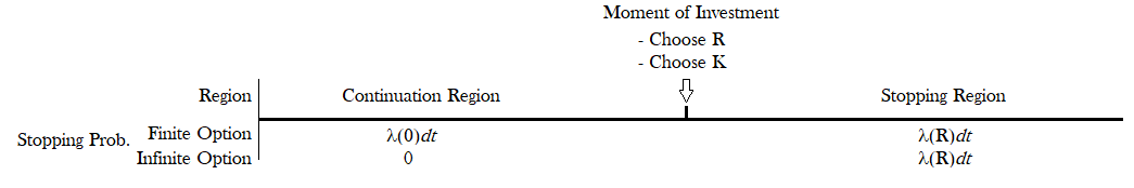
We consider two situations, one in which the lifetime of a project is finite and option to invest is infinite, and one in which the lifetime of a project is finite and the option to invest is finite as well. To obtain a finite option to invest, we add the probability that a project stops with  to the continuation region. In Figure 1 we can see a visualization of the investment timeline. In this latter case, the option to invest can disappear if a firm waits too long to invest in a project. Think of it as if a new external product is launched on the market by another investor and that causes the product of the initial investor to be useless. For example, a videotape player became almost useless when DVDs entered the market.
The value of a monopolist in the case of a finite option to invest is shown in Proposition 1.
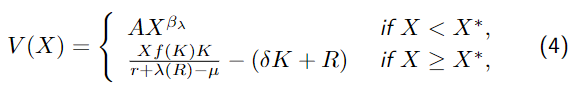
where A is an unknown constant, and

The optimal investment decision of a monopolist in the situation where project life is finite and the option to invest is
finite can be seen in Proposition 2.
Proposition 2. The optimal investment threshold equals

where the optimal investment size satisfies

and the optimal amount of money to invest in an R&D laboratory satisfies

In order to gain more intuition on the implications of Proposition 2, we will visualize what happens to the optimal decision
with respect to the stochastic drift rate
X*
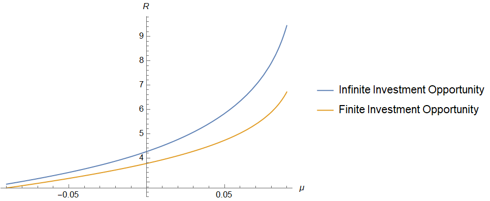
R
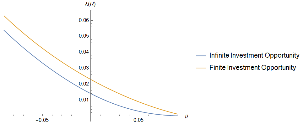 , optimal investment size , optimal R&D investment size , and creative destruction
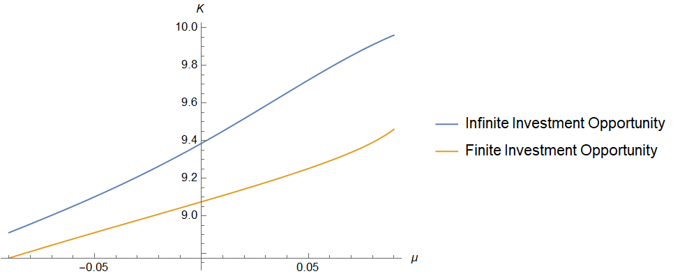
  as a function of . Parameter values are
  .
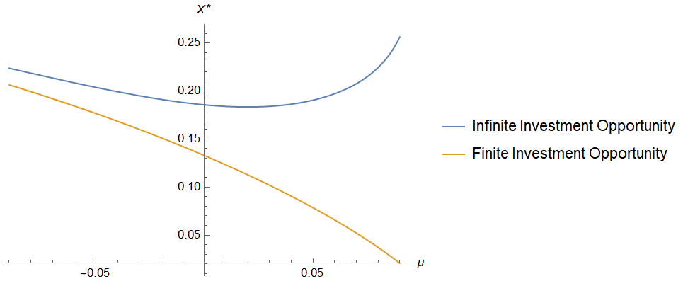
.Note that we also added the optimal investment decision when considering an infinite investment opportunity in the figure. We can see the difference between both the finite case and the infinite case clearly in Figure 2a. It is noticeable that for small , the investment threshold is decreasing, while for larger , the investment threshold is increasing in . In the finite option to invest case, a firm will always accelerate its investment when the trend is higher. We have to take into account that a project can stop before a firm even invested in it, which is why it seems plausible that the higher the trend, the earlier a firm wants to invest in the project so a firm cannot lose its option. Likewise, if the trend is very low, it is not that unfortunate if the option to invest disappears and therefore a firm is willing to wait longer to invest in a product. In equation (9) you can find the comparative statistics analysis of Figure 2a for the finite option to invest situation.

Balter, Huisman, and Kort (2021) distinguish three effects: the net present value (NPV) effect  , option effect
  and quantity effect
  . The NPV effect is the effect of an increase in the net present value of an investment when the trend is higher, whereas the option effect causes the value of the option to invest to increase under a higher trend. The quantity effect is the effect where a larger drift rate causes a firm to invest more in capacity, which also increases the total investment costs and therefore the investment threshold. By adding an extra decision to the model we found a fourth effect; the R&D effect
  . The R&D effect accelerates a firm’s investment together with the option effect and the quantity effect, while the NPV effect does the exact opposite.
To conclude, in this article we have started investigating an additional decision on the investment, by introducing the possibility to invest in an R&D laboratory at the moment of investment. With an R&D laboratory a firm can update its product throughout the time it is active in the market to extend the expected lifetime of the product. We find that a new effect arises with the introduction of a new decision on investing in an R&D laboratory.
References
Aguerrevere, F. (2003). “Equilibrium Investment Strategies and Output Price Behavior: A Real-Options Approach”. In: The Review of Financial Studies 16.4, pp. 1239–1272.
Avram, E. et al. (2009). “Investment decision and its appraisal”. In: DAAAM International 20.1, pp. 1905–1906.
Balter, A.G, K.J.M Huisman, and P.M Kort (2021). “New insights in capacity investment under uncertainty”. In: Working Paper.
Dixit, A. and R. Pindyck (1994). “Investment under Uncertainty”. In: Princeton University Press.
Huisman, K.J.M and P.M Kort (2015). “Strategic capacity investment under uncertainty”. In: The RAND Journal of Economics 46.2, pp. 376–408.