Humanitarian logistics optimization
Humanitarian logistics is often described as the process of planning, implementing, and controlling the flow and storage of goods/information, intended to reduce the suffering of vulnerable people, from the point of producing to the point of consumption [2]. In this article we introduce two challenges that occur in humanitarian logistics. The first problem belongs to the class of preparations in order to respond to disasters. The second problem appears in the (immediate) response phase after a disaster hit a region.
Written by: Valentijn Stienen
Introduction
As you can imagine, the field of humanitarian logistics has a very broad scope. Therefore, the following four categories within humanitarian logistics are often distinguished [3]:
- The mitigation phase refers to the precautions that are taken to mitigate specific disasters. E.g., building reliable infrastructure.
- The preparation phase refers to the operations that occur during the period before a disaster strikes. E.g., storing additional relief items in disaster prone areas.
- The response phase refers to the actions taken within the first few days after a disaster occurred. E.g. providing first aid (food, supplies, medicine) to people that are stuck in a flooded area.
- The development phase of a disaster consists of the operations done in the months/years after the disaster occurred. E.g. long-term recovery operations.
In this article, we treat two different optimization problems related to these phases. First, a problem is discussed which belongs to the preparation phase. We determine optimal locations for pre-positioning relief items. The second problem is related to the response phase. Here, we try to optimize decisions regarding the routing of relief items to affected people. We incorporate the high uncertainty about the (road) conditions in the disaster area.
Optimal pre-positioning locations
When disaster strikes an area, international assistance (e.g., international relief organizations) is often requested to help responding and recovering from the disaster. This response can be characterized by the dispatch of relief items (e.g., tents, tarpaulins, food or hygiene kits) to the affected regions. To enhance response capabilities, humanitarian organizations often make use of pre-positioning their inventory. This may significantly reduce the time it takes to deliver emergency items to the affected people. However, it is often not easy to store goods anywhere in the world.
This is where Humanitarian Logistics Service Providers (HLSP) come into play. A HLSP offers services to humanitarian organizations that improve the supply chain of these organizations. For instance, an HLSP may offer storage locations in specific regions of the world. One of the largest HLSPs is the United Nations Humanitarian Response Depot (UNHRD). The UNHRD offers free storage space to humanitarian organizations (for free) in multiple locations across the globe. In this way, organizations can implement these locations in their pre-positioning network. Besides that, the UNHRD offers to ship the stored relief items to the affected regions on behalf of the humanitarian organizations. This may result in lower costs due to bulk shipments/flights. The first question we now try to answer is how to distribute three HLSP depots across the world in an optimal way.
We determine the optimal distribution of depots based upon historical data from EM-DAT [1]. We try to find depots, which are located in an optimal way for the historical disasters. In particular, we assume that the depots store relief items intended for countries with a Human Development Index (HDI) smaller than 0.8.
This problem can be formulated as a basic Facility Location Problem (FLP). Let  be the set of possible depot locations and let
  be the set of disasters that will be assigned to depots. We denote the cost of supplying disaster
  from possible hub locations
  by
by  . Furthermore, let
  be a binary variable that indicates whether depot is opened (
 ). Finally, let
  be a non-negative variable indicating whether disaster is supplied by (open) depot . Then the FLP can be described as in Model 1.
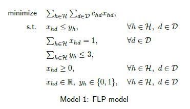
The first constraint ensures that disasters can only be supplied by open depots. The second constraint makes sure that each disaster is supplied by a depot and the third constraint bounds the total number of open depots to three. There are some additional pre-processing steps required to solve this model. To determine the set of possible depot locations , we select locations that both contain a large harbor and airport. Both restrictions ensure that relief items get dispatched as easy as possible. The set of disasters contains all disasters reported in the EM-DAT between 2017 and April 2019, which affected at least 100 people. Finally, the cost of assigning a disaster to a depot is computed as follows. We assume that part of the delivery to a disaster is done via sea and part is done with aircraft (the immediate response). Figure 1 illustrates the costs involved.
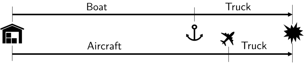
This means that we first map each disaster to its nearest harbor and airport. Subsequently, we can determine the total transportation cost by summing up the total truck/boat/aircraft costs.
Solving this model gives us the distribution of depots that generates the least amount of transportation costs. The total minimized cost is $1.53B. However, in humanitarian context, costs do not solely determine the quality of the solution. Another important factor for pre-positioning depots is the maximum response time. This is a quantity that is supposed to be minimal as well. Let  be the response time when disaster is assigned to depot . Then, the second objective of the FLP is minimizing:

Now, our focus becomes finding the Pareto front of the FLP with the two objectives. First, we solve the FLP only minimizing the maximum response time. The solution is a distribution of depots from which humanitarian organizations can respond within 28 hours. Next, we minimize the transportation cost while ensuring that the maximum response time equals 28. The result is a cost of $1.98B. Computing the minimal cost for an increasing response time (in hours) results in the Pareto front shown in Figure 2.
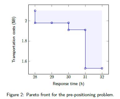
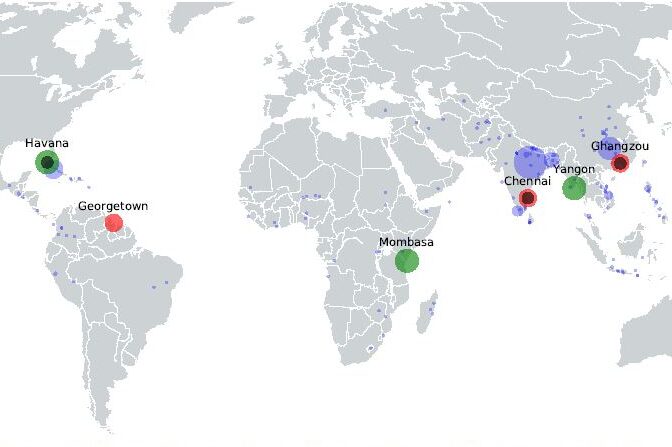
From Figure 2, we can see that there exist 3 strongly Pareto optimal solutions. For clarity, we visualized these three solutions in Figure 3. The blue dots represent the considered disaster locations. Disasters with a high number of affected people are displayed with a larger dot.
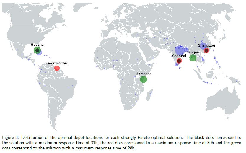
As we expect, allowing for a higher maximum response time results in optimal depot locations which are moved to the regions where disasters affected the largest amount of people.
Routing relief items
Next, we discuss the problem of routing relief items in a disaster area in which there is uncertainty in the road conditions. We will work through a simple example to show how decisions can be optimized. Consider the situation in Figure 4.
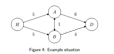
We want to deliver relief items from the harbor ( ) to the disaster area (
 ). We can deliver via two additional cities,
  and
and  . The edge labels represent the distances between nodes. The jagged edge between and means that we are currently not sure whether this road is destroyed or not. We assume that we can use this road with probability 0.5. Finally, we assume that we are allowed to decide the direction of the truck each time it visits a node.
When ignoring the probabilities, the shortest path solution ( ) is optimal (length 9). To incorporate the probabilities, we seek a strategy that minimizes the expected length of the route to the disaster site. We model the situation as a Markov Decision Process (MDP) as is done in [4].
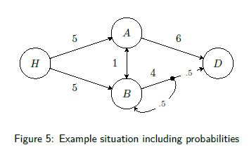
Figure 5 is a new representation of the example in which the jagged edge ( ) is replaced with an edge containing a dot in the middle. This edge can be interpreted as follows. If we choose to traverse edge , we always cover a distance of 4. Then, we either end up in or in (when the road turns out to be destroyed), both occurring with 50% probability.
Let  be the state space of the MDP. Furthermore, in each state
  we have a set of actions
  . For instance,
  . Next, we assign a value to each state that represents the expected minimal distance from state to the disaster site . I.e.,
  and the values for the remaining states can be written as follows:
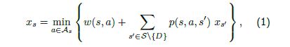
where  denotes the distance traveled when action
  is chosen while in state .
  is the probability of ending up in state
  starting in state when choosing action . If the truck is currently in state , then the optimal action is the that attains the minimum in (1). To find these values we can solve the following linear program:

Note that the values of states can change over time when information about road conditions becomes available. This means that when new information becomes available, the values need to be updated.
Next, we discuss the numerical results for the example introduced before. When the truck starts in the harbor, the values of the states (minimal expected distances to ) are  ,
,  and
and  . For instance, if we start in , we need to traverse at least an expected distance of 6 to reach . To find the current optimal decision, we determine for each state the action that results in the minimum value, i.e.,
 . First, we drive a distance of 5 (
 ). Then, we expect to drive
  . Total: 11.
 . First, we drive a distance of 5 (
 ). Then, we expect to drive
  . Total: 13.
Minimizing the total expected length results in choosing to go from to . Once arrived in another decision has to be made. Suppose that now it has become known that the road between and is open. This means that we update the values of the states,  ,
,  and
and  . Again, we compare,
 . First, we drive a distance of 6 (
 ). Then we arrive at . Total: 6.
- . First, we drive a distance of 1 (
 ). Then, we expect to drive
  . Total: 5.
Hence, we choose to go to . Similarly, our last choice will be to go from to . In short, the path we traversed is  . This path is not the shortest path, but it took into account that the edge might have been destroyed.
Conclusion
A challenging part of doing research in the field of humanitarian optimization is to provide solutions to problems that can actually be used by humanitarian organizations. On the one hand, the problems which are addressed need to be aligned with the problems faced by the humanitarian organizations. On the other hand, the solutions that are found need to be accessible and implementable by humanitarian organizations.
The first project described is done is close cooperation with the UNHRD. In this study we include additional factors specific for UNHRD. For instance, we consider the political difficulties of establishing a depot in a country. Furthermore, we consider other scenarios such as optimally expanding their current network, by allowing one hub to be added to their current network. For the second study, we are developing more realistic models. For instance, using adjustable robust optimization, we try to include information about when road conditions are examined and reported.
References
[1] EM-DAT: The Emergency Events Database – Université catholique de Louvain (UCL) – CRED, D. Guha-Sapir – www.emdat.be, Brussels, Belgium
[2] Thomas, A.S. & Kopczak, L.R. (2005). From logistics to supply chain management: the path forward in the the humanitarian sector. Fritz Institute, 15, 1-15.
[3] Tomasini, R., Van Wassenhove, L. (2009). Humanitarian logistics . Springer.
[4] Randour, M., Raskin, J. F., \& Sankur, O. (2015). Variations on the stochastic shortest path problem. International Workshop on Verification, Model Checking, and Abstract Interpretation, 1-18.