Math wrapping up misdemeanor

A dark alley, a sinister park, or an abandoned manor; crime is everywhere and the delinquents are far from being caught. Police officers are busy day and night to find and catch notorious killers, not even mentioning the fact that it needs to be proven that the villain in question is indeed the culprit. Little did these officers know that their rescue would lie in a field of science which, at first sight, seems to be as unrelated to solving crime as televisions are related to a peanut butter sandwich, namely mathematics.

Yes, indeed. Mathematics is a major factor in current day crime fighting. Some people may already know that math plays an important role in crime fighting because of the hit show “NUMB3RS”. For those of you who have not heard about the series, it is about a police officer named Don Eppes and his brother Charlie, a mathematical genius. Together, they solve crimes in the streets of Los Angeles. Enough about the series, though. I shall put several ways in which math is used in current day crime fighting forward and shall show you the magical world of mathematics taking care of misdemeanor.

Detecting the delinquent:
Always bothering the minds of crime fighters is the location of the perpetrator. They seem to be able to determine an area in which the culprit should be living, but are rarely able to pinpoint the exact location. This is where we encounter our first application of mathematics in crime fighting, Rossmo’s formula.

Assume that the city is partitioned in a grid of little squares, much like a table, with i rows and j columns. In this formula, p_ij denotes the probability that the villain resides in the location in row i and column j and c denotes the total number of crimes.

Firstly, one calculates the distance from the center point of a square in row i and column j (x_i,y_i) to the square of each crime scene, namely (x_n,y_n), where n denotes the number of the crime, i.e., n=1 means “first crime”, n=2 means “second crime”, etcetera. This whole bit is denoted by |x_i – x_n|+|y_j– y_n|. Rossmo’s formula uses this expression in two ways. In the first term, with ϕ in the numerator, the expression is put in the denominator and is raised to the power f. How f will be determined depends on what works best when the formula is checked against data on past crime patterns. This term tells us that the probability of crime scenes decreases as distance increases.

Secondly, the travelling distance is used with regards to the so-called buffer zone, the area around the place where the criminal lives where they commit little to no crimes, as the chance to get caught is higher. In the second fraction, the distance is subtracted from 2B, where B is chosen to describe the size of said buffer zone. This means that the subtraction will give us smaller answers when the distance increases and such, after raising this part in the denominator to another power, namely g, you will get larger results. These two parts together express that, as you move through the buffer zone, the probability of crimes being committed first increases and then decreases. We combine these parts by inserting the well-known sum sign Σ. The number ϕ will place more weight on one term or the other. When increasing ϕ, there will be more weight on the decreasing probability as distance increases. A smaller ϕ will put more weight on the effect of the buffer zone.

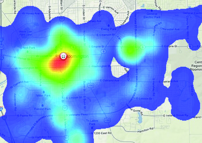
When having all probabilities p_ij calculated, we can construct a hot zone map, as seen in Figure 1. The red part of the map shows us the places where the probability that the perpetrator lives in that area is highest. Moving out, this probability decreases and is denoted by green and blue colorings.

Proving the perpetrator’s guiltiness:
One of the most crucial parts of evidence is DNA. Officers find traces of DNA often at crime scenes, where it can be found as puddles of blood, hairs lying on the floor or the semen on the bed. Thinking about it, the mathematical aspect of DNA profiling seems obvious. Again, it is probabilities that play a role, as in many parts of crime fighting.

Most people have probably heard of the term CODIS, the name of the database of DNA samples of the FBI. CODIS is the abbreviation for Combined DNA Index System. The CODIS DNA database consists of four categories of DNA records:

1. Convicted Offenders: DNA identification records of persons convicted of crimes.
2. Forensic: Analyses of DNA samples recovered from crime scenes.
3. Unidentified Human Remains: Analyses of DNA samples recovered from unidentified human remains.
4. Relatives of Missing Persons: Analyses of DNA samples voluntarily contributed by relatives of missing persons.

CODIS contains over three million records of convicted offenders. The DNA profiles in CODIS are based on thirteen specific loci(also called sites), which were chosen because they show considerable variation among people. When two randomly chosen samples match in all or a lot of the thirteen loci selected for the CODIS system, it is safe to say that the probability that these samples have come from two totally unrelated people is nearly zero. Therefore, DNA identification is extremely reliable and is used often in practice.

Let us first consider a DNA profile based on only four loci. It is generally accepted that the probability that someone would match a random DNA sample at any one locus is roughly 1/10. It has been derived from empirical studies of allele frequencies of large numbers of samples that 1/10 is a good representative number. Hence, the chance that someone would match a random DNA sample of four loci would be about 1/10,000. When using this number with regards to all thirteen loci used in CODIS, then the probability of matching some given DNA sample at random in the population will be (1/10)¹³, one in ten trillion. This number is known as the random match probability, or RMP for short. As devoted econometricians, we know that this rule only holds when the probabilities are independent of each other. There has been a lot of debating whether or not the probabilities are actually independent, but this issue has faded over time and has almost completely died away. Some people will still doubt whether the generally accepted probabilities are actually valid, but nevertheless, it is surely the case that when someone’s DNA profile matches on all thirteen loci implemented in the CODIS system, that the identification is virtually certain, assuming that the match was deduced by a process consistent with the randomness regarding the RMP. However, the math is quite sensitive to how well that assumption is satisfied.

In reality, the authorities find evidence that ties a certain someone to the currently running case, but they fail to deliver an identification with enough certainty to obtain a conviction. However, when CODIS points out that this person has a match with said DNA profile on (nearly) all thirteen loci, then we can safely assume that a match has been found, although we must not rule out the fact that the assumed culprit has relatives that closely match his or her DNA profile. Sometimes, siblings are separated at birth and these individuals may be unaware that they even have a sibling. Hence, this possibility must always be investigated.

Convicting the culprit:
After these two steps have been taken, there is one last step on the road of crime fighting: convicting the criminal for his deeds. The authorities take the culprit to court, where a jury or judge will decide whether or not the person is guilty of committing the crime. We have seen that mathematics can provide a DNA profile match, but there is far too little evidence to prove an individual guilty. In court, there is often visual evidence presented, such as photographs. If you have ever seen photographs taken from afar, you can confer that they are almost never really clear. This is where mathematics takes a peek around the corner once again. Math is able to virtually enhance photographs to determine the actual validity of such a picture and whether it actually shows that the person in question is indeed guilty. The key technique to this method is segmentation: splitting up the image in regions that correspond to distinct objects, parts of objects or persons in the original picture, such as objects in the background.

Digital images are displayed as rectangular arrays of pixels, each pixel having a unique pair of coordinates (x,y). Therefore, we can view any edge or line in the picture as a curve. As we know, we can define curves by equations. We all know that a straight line of pixels would then satisfy an equation of the form y = ax + b. We can thus try and identify collections of pixels of (roughly) the same color that satisfy such an equation. Of course, this equation will not be exact and hence we must allow for a reasonable amount of approximation, such that the equation is satisfied.

When assuming a black-and-white image, this picture is just a function f from a given rectangular space into the real unit interval, namely [0,1]. If f(x,y) = 0, then the pixel with coordinates (x,y) is colored white. Also, if f(x,y) = 1, then the pixel with coordinates (x,y) is colored black. For all other cases, f(x,y) denotes a shade of gray. The greater the value of f(x,y), the darker the shade of gray. Since we can denote this formula so easily, it is generally also easier to enhance black-and-white images than to enhance colored pictures. Still, it is quite difficult to explain and we will not go into more detail here. However, one man did delve deeper into this problem.

There once was a man named Leonard Rudin, who asked himself certain questions, such as “Why do we see a single point on a piece of paper?”, “How do we see edges?”, “Why is a checker board pattern with many squares so annoying to the eye?” or “Why do we have difficulty understanding blurry images?”. When he linked these questions to the corresponding function f(x,y), he quickly found out what the significance of singularities in the function is. Because of this revelation, he focused his attention on finding a particular way to measure the closeness of a particular function to a given image, the so-called total variation norm. The details of his research are once again hard to explain and highly technical, but they are not required to be mentioned here. Do read into it, though, if you are interested. Due to his research, Rudin managed to develop computational techniques to restore images using what is now called the total variation method, which uses Euler-Langrange PDE minimization on the total variation function.

Case concluded:
By now you know some of the most prevalent methods which are used for catching culprits, proving them to be the perpetrator and convicting them for the crook that they are. It is highly surprising to see that mathematics are so closely related to this common apparition, although at the same time, one could have expected this. Mathematics, after all, is currently one of the most used sciences. Try and think of a subject where mathematics is not used. Even in the assumed core science of physics, mathematics is used. Hence, mathematics is everywhere, haunting all criminals, so do not even dare to steal that one candy bar you crave or to cheat on your exams.

Text by: Mike Weltevrede