Epidemics, Vaccines and Mathematics

August 8, 2019February 24, 2021 Nekst-Online 235 Views Epidemics, SIR model, Vaccines

Infectious diseases have had an enormous impact on the course of human history. Various epidemics have killed hundreds of millions of people, and some diseases have been responsible for the depopulation of large areas. One would expect that reliable vaccines for deadly diseases are met with nothing but approval and appreciation. Instead, vaccination rates are dropping recently due to controversy and the spread of misleading information. This raises the question: what can math tell us about epidemics and vaccination?
Written by: Stefan ten Eikelder

The antivax community has caused quite a stir in the world of epidemiology. A 1988 British study falsely concluded that the MMR (measles, mumps, and rubella) vaccine caused autism in 8 out of 12 patients in the study. Later, it turned out that the researcher involved falsified the data and the results were debunked. Nevertheless, the results sparked an increase in the antivax movement, and the connection between vaccines and autism is still upheld by many people. An increasing number of people who refuse to vaccinate their children leads to an increase in the probability of new epidemic outbreaks, and is thus cause for major concern among healthcare experts.

We refrain from the political discussion, and focus on the math. We will introduce the most popular mathematical model for the spread of infectious diseases, and we will analyze how vaccinations can prevent an epidemic and eradicate the disease.

The SIR model

In 1927, the seminal work of Kermack and McKendrick [1] introduced the SIR model. This is a so called compartmental model, as it splits the population in three groups/classes: Susceptible (S), Infected (I) and Recovered (R). An individual is susceptible if (s)he has not (yet) been exposed to the disease, infected if currently carrying the disease, and recovered if they have cleared their infection. It is assumed that individuals who have recovered have gained immunity to the disease. An individual in class S moves to class I once infected, and an individual in class I moves to class R once they have fought off the disease.

The standard SIR model is deterministic, and assumes a homogeneous population. Hence, the change in any compartment size can be described by a partial differential equation (PDE). Let $N$ denote the population size and let $X$ , $Y$ and $Z$ denote the number of individuals in classes S, I and R, respectively. The alert reader will notice that we implicitly assume that the infectious disease does not have a substantial mortality risk. Since an analysis of deadly diseases is more complicated, we focus on benign (non-deadly) diseases.

Suppose an individual makes $k$ contacts with other individuals per unit of time. Then, during a small time period of length $\delta t$ , the individual has contact with $k Y/N \delta t$ infected people. Suppose that the probability of succesfull disease transmission is $c$ . Then, a susceptible individual does not get infected during this time period with probability

$1 - \delta q = (1-c)^{\frac{kY}{N \delta t}},$

so $\delta q$ is the probability of infection for these contacts. With an extra definition, $\beta = -k \log (1-c)$ , we can rewrite the previous equation to

$\delta q = 1 - e^{\frac{-\beta \delta t Y}{N}}.$

Now, we expand the right hand side using the Taylor expansion and divide both sides by $\delta t$ . Subsequently, we take the limit $\delta t \rightarrow 0$ to find

$\frac{dq}{dt} = \frac{\beta Y}{N}.$

This is the rate at which a susceptible individual gets infected. Then the rate of transmission for the entire susceptible class is given by

$\frac{dX}{dt} = \frac{-\beta X Y}{N}.$

With slight abuse of notation, we let $S$ , $I$ and $R$ indicate the fraction of the population in these classes, so $S + I + R = 1$ . Then the transmission rate for the S class is

$\frac{dS}{dt} = -\beta IS,$

the parameter $\beta$ is known as the transmission rate parameter, and $1/\beta$ can be interpreted as the time between contacts with disease transmission. The SIR model is given by

(1a) $\begin{equation*} \frac{dS}{dt} = -\beta SI \end{equation*}$

(1b) $\begin{equation*}\frac{dI}{dt} = \beta SI - \gamma I \end{equation*}$

(1c) $\begin{equation*}\frac{dR}{dt} = \gamma I, \end{equation*}$

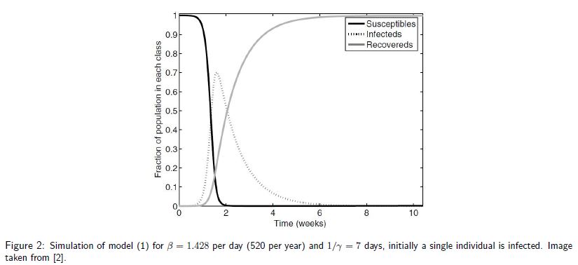
where $\gamma$ is the recovery rate of infected individuals. That is, $1/\gamma$ is the duration of an infection. The model 1a cannot be solved analytically. Nevertheless, we can simulate the progression of the disease. An example is displayed in Figure [2], where initially a single individual is infected and at the peak $70\%$ of the population is infected. It is important to note that in model 1a the disease will eventually die out due to the fixed population size.

The threshold phenomenon

Despite the simplicity of the SIR model, it provides a crucial insight into the factors that determine whether or not there will be a proper epidemic outbreak. We can rewrite 1b to

$\frac{dI}{dt} = I(\beta S - \gamma).$

Then, if $\frac{\beta}{\gamma} S(0) > 1$ we have $\frac{dI}{dt}(0) >0$ , so the number of infected people initially increases. The ratio $\frac{\beta}{\gamma}$ is known as the basic reproductive number $R_0$ . This is the number of new infections created by an infected individual. The basic reproductive number plays a crucial role in epidemiology for the following reason. For many infectious diseases it is reasonable to assume that initially the entire population (except the first infected individual) is susceptible, so $S(0) = 1-\epsilon$ . Then the disease spreads if $R_0 \geq 1$ and dies out if $R_0 < 1$ . 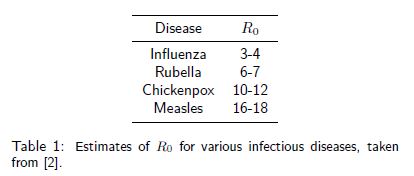This is known as the threshold phenomenon, first discovered by [1]. The higher $R_0$ , the faster the disease spreads and the hard it is to control. Table 1 shows $R_0$ estimates for various diseases.

Modeling life and death

Before we move to vaccinations, we add birth and (non-disease related) death dynamics. For our simple deterministic model, we assume a lifespan of $1/\mu$ years, so $\mu$ is the rate of birth and death. Newborns enter the system as susceptible, and deaths can occur in all classes. The SIR model with demographics now reads

(2a) $\begin{equation*} \frac{dS}{dt} = \mu - \beta SI - \mu S \end{equation*}$

(2b) $\begin{equation*} \frac{dI}{dt} = \beta Si - \gamma I - \mu I \end{equation*}$

(2c) $\begin{equation*} \frac{dR}{dt} = \gamma I - \mu R. \end{equation*}$

We can derive the basic reproductive number $R_0$ for this model in a similar fashion as in the previous section:

$R_0 = \frac{\beta}{\gamma + \mu}$

Compared to model (1), this model allows for analysis of the long term behavior of the disease in the population, due to the inclusion of birth-death dynamics. Two equilibria can be determined, by simply setting the right-hand side expressions in (2) to zero. For 2b we find that either $I^{\ast} = 0$ or $S^{\ast} = \frac{\mu + \gamma}{\beta}$ . The former leads to the disease-free equilibria:

$(S^*,I^*,R^*) = (1,0,0),$

and the latter leads to the endemic equilibria:

$(S^*,I^*,R^*) = \left( \frac{1}{R_0},\frac{\mu}{\beta}(R_0 - 1),1-\frac{1}{R_0} - \frac{\mu}{\beta}(R_0-1) \right).$

Because the population variables must be nonnegative, the endemic equilibria is only possible if $R_0 \geq 1$ . Hence, we again observe the threshold phenomenon.

Vaccinations to the rescue

Suppose a fraction $p$ of the population is vaccinated at birth via a so-called pediatric vaccination program and that vaccination confers lifelong immunity. This can be modelled by letting vaccinated newborns enter the system in the recovered class (which is essentially an immune class) instead of in the susceptible class. Non-vaccinated newborns still enter the system in the susceptible class. The SIR model with vaccination reads

(3a) $\begin{equation*} \frac{dS}{dt} = \mu (1-p) - \beta SI - \mu S \end{equation*}$

(3b) $\begin{equation*}\frac{dI}{dt} = \beta SI - \gamma I - \mu I \end{equation*}$

(3c) $\begin{equation*}\frac{dR}{dt} = \gamma I + \mu p - \mu R. \end{equation*}$

We are now in position to analyze the influence of the vaccination rate $p$ . In [3] the following variable substitution is proposed: $S = S'(1-p)$ , $I = I'(1-p)$ and $R = R'(1-p) + p$ . Then model (3) is equivalent to

(4a) $\begin{equation*} \frac{dS'}{dt} = \mu - \beta (1-p)S'I' - \mu S' \end{equation*}$

(4b) $\begin{equation*}\frac{dI'}{dt} = \beta (1-p)S'I' - (\gamma + \mu)I' \end{equation*}$

(4c) $\begin{equation*}\frac{dR'}{dt} = \gamma I - \mu R. \end{equation*}$

One can recognize that (4) in fact has the same structure as model (2), the only difference is that $\beta$ is replaced by $\beta (1-p)$ . Let $R_0'$ denote the vaccination corrected basic repopulation number. Then we must pick the fraction $p$ such that $R_0'$ is below 1. With $\beta$ replaced by $\beta (1-p)$ , we get

$\frac{\beta (1-p)}{\gamma + \mu} < 1 \Leftrightarrow p > 1 - \frac{1}{R_0}.$

Hence, to eradicate a disease, it is crucial to vaccinate at least a fraction $p_c = 1- R_0^{-1}$ of the newborns. Of course, vaccinating more than $p_c$ will make sure the disease is eradicated more rapidly. It is now straightforward to calculate the critial proportion $p_c$ for the diseases in Table1. The fact that it is not neccesary to vaccinate all newborns is known as herd immunity: non-vaccinated (susceptible) individuals are protected from infection because they are surrounded by a sufficient number of vaccinated individuals.

Reality: Heterogeneity, imperfect vaccines and noise

The simple SIR model provides some fundamental insights in the spread of disease and the influence of vaccinations. However, it makes quite a few assumptions, which limit the direct applicability of the model. In particular, it assumes a non-deadly disease. Furthermore, it assumes a homogeneous population (with fixed lifespan and infection duration), vaccines providing lifelong immunity and a deterministic disease spread. Many variations on the SIR model have been developed to deal with these limitations [2]. In particular, stochastic differential equations are a proper tool to add many of these components to the model.

Math is at the heart of epidemiology, and provides crucial insights into the effects of various vaccination strategies. In the current political debate on vaccines, its importance will probably not die out soon.

References

[1] W.O. Kermack and A.G. McKendrick (1927). A contribution to the mathematical theory of epidemics. Proceedings of the Royal Society of London. Series A 115(772) 700–721.
[2] M.J. Keeling and P. Rohani. (2008) Modeling infectious diseases in humans and animals. Princeton University Press
[3] D.J.D. Earn et al. (2000). A simple model for complex dynamical transitions in epidemics. Science, 287(5453), 667–670.

The SIR model

The threshold phenomenon

Modeling life and death

Vaccinations to the rescue

Reality: Heterogeneity, imperfect vaccines and noise

References

You May Also Like

Many Thanks to our Professor, Colleague and Friend

The Working Holiday Visa

The Optimal Wine Adventure